3D multi-physics simulations
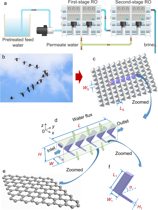
In typical spiral wound membrane systems, each module includes more than 1 million feed spacer cells. Therefore, it is computationally impractical for simulation of each membrane module using the 3D multi-physics model. Fortunately, previous work43,52 indicated that “periodic fully-developed” flow and mass transfer reached in just several cells. Therefore, it is possible to capture the local hydrodynamic and transport characteristics using a computational domain that consists of a few feed spacer cells. The average mass transfer coefficient and the axial pressure drop per unit length at various locations along feed direction are calculated by changing the feed velocity at the inlet of the computational domain. In this work, the established 3D multi-physics model (direct problem) considers the fluid flow (1) and mass transport (2) in five unit cells (\(\varOmega\); Fig. 1d) that can be mathematically described as
$$\left\{\begin{array}{ll}\rho ({\mathbf{u}}\cdot \nabla ){\mathbf{u}}-\nabla \cdot [-P{\mathbf{I}}+\mu (\nabla {\bf{u}}+{(\nabla {\bf{u}})}^{{\rm{T}}})]=0,\,&{\rm{in}}\,\Omega ,\\ \nabla \cdot (\rho {\mathbf{u}})=0,\,&{\rm{in}}\,\Omega ,\end{array}\right.$$
(1)
and
$$\nabla \cdot ({D}_{{\rm{s}}}\nabla c)-{\bf{u}}\cdot \nabla c=0,\qquad\qquad\,{\rm{in}}\,\Omega$$
(2)
respectively. The location of the inlet cross-section for the computational domain (Fig. 1d) is chosen arbitrarily to guarantee generality. ρ, μ, \({D}_{{\rm{s}}}\) are fluid density, viscosity, and salt diffusivity. More detailed information, e.g., boundary conditions, model parameters for the multi-physics model was reported in our previous work.39 Pressure drop per unit length \(\frac{\Delta {P}_{{\rm{c}}}}{L}\) is calculated by
$$\frac{\Delta {P}_{{\rm{c}}}}{L}=\frac{{P}_{{\rm{in}}}-{P}_{{\rm{out}}}}{L}$$
(3)
where \({P}_{{\rm{in}}}\) and \({P}_{{\rm{out}}}\) denote average pressure at inlet and outlet respectively, and L is the length of computational domain (Fig. 1d). The Darcy friction factor is estimated by29
$$f=\frac{2{D}_{{\rm{H}}}\varDelta {P}_{{\rm{c}}}}{\rho {\bar{u}}^{2}L}.$$
(4)
The hydraulic diameter, \({D}_{{\rm{H}}}\) is calculated by the formula from the literature.43 The Sherwood number, \(Sh\) can be obtained using
$$Sh={\bar{k}}_{{\rm{m}}}\frac{{D}_{{\rm{H}}}}{{D}_{{\rm{s}}}}.$$
(5)
The cell-average mass transfer coefficient on membrane walls (Fig. 1d), \({\bar{k}}_{{\rm{m}}}\) is estimated by
$${\bar{k}}_{{\rm{m}}}=\frac{{\int }_{0}^{L}{\rm{d}\it{y}}{\int }_{0}^{W}(\frac{-{D}_{{\rm{s}}}}{{c}_{{\rm{r}}}-{c}_{{\rm{w}}}}\cdot \frac{\partial c}{\partial z}){\rm{d}\it{x}}}{{\int }_{0}^{L}{\rm{d}\it{y}}{\int }_{0}^{W}{\rm{d}\it{x}}}.$$
(6)
\({c}_{{\rm{r}}}\) denotes solute concentration at bulk of retentate that is equal to inlet concentration (\({c}_{0}\)). \({c}_{{\rm{w}}}\) is solute concentration at membrane wall.
Module design
The inverse design problem of feed spacer can be mathematically expressed as
$$\begin{array}{c}\mathop{\min }\limits_{{{{\bf{\upbeta}}}}_{1}}{F}_{1}\\ s.t.\,{{{\bf{H}}}_{1}=\bf{0}},\end{array}$$
(7)
where the design variables are spacer geometric parameters, \({\bf{\upbeta}}_{1}=[{L}_{1},\,{W}_{1},\,{H}_{1},\,\alpha ,\,{L}_{\rm{S}},\,{W}_{\rm{S}}]\) (Fig. 1c, d, f). The inlet cross-flow velocity is fixed (\(\bar{u}\) = 0.1 m s−1). The optimized spacer parameters (\({\bf{\upbeta }}_{1,{\rm{opt}}}\)) can be obtained (Supplementary Fig. 2) by solving 3D nonlinear partial differential Eqs. (1, 2; \({{\bf{H}}}_{1}\,=\,\bf{0}\)) constrained optimization problem. For the objective function of \({F}_{1}=\frac{(\Delta {P}_{{\rm{c}}}/L)/(\Delta {P}_{{\rm{c}},0}/{L}_{0})}{{({\bar{k}}_{{\rm{m}},{\rm{imp}}}/{\bar{k}}_{{\rm{m}},{\rm{imp}},0})}^{\beta }}\), the \(\Delta {P}_{{\rm{c}}}/L\) and \(\varDelta {P}_{{\rm{c}},0}/{L}_{0}\) denote axial pressure drop per unit length for the designed membrane module of this work and the conventional module respectively. The detailed geometric parameters for the latter one were reported in our previous work.45 \({\bar{k}}_{{\rm{m}},{\rm{imp}}}\) and \({\bar{k}}_{{\rm{m}},{\rm{imp}},0}\) denote cell-average mass transfer coefficients using the impermeable wall model for the designed and conventional modules respectively that can be converted to the cell-average mass transfer coefficient on permeable wall using reported relations.53 Detailed quantitative analysis indicated that the estimated error using both permeable and impermeable wall models is less than 10% even under a high water flux condition of 200 lmh at system inlet while the latter requires significantly shorter computational time. The power exponent (β) is used to control the tradeoff between flow resistance and mass transfer. The genetic algorithm toolbox, GATBX38 is used to solve the optimization problem due to its superior performance on global convergence.
Based on the optimized spacers (β = 4, 6, 8), we further obtain the correlations of Sherwood number and Darcy friction factor
$$S{h}_{{\rm{imp}}}=kR{e}^{t},$$
(8)
$$f=\mathop{\sum }\limits_{i=1}^{8}({a}_{i}R{e}^{i}+{b}_{0}),$$
(9)
using the CFD simulations with various Reynolds numbers (Re = 50, 62.5, 75…1,000) (Supplementary Fig. 2). The cross velocity (\(\bar{u}\)) is calculated by
$$\bar{u}=\frac{\mu Re}{\rho {D}_{{\rm{H}}}}.$$
(10)
These correlations (8) and (9) enable a quantitative description of mass transfer and flow resistance, which can be used for system design.
System modeling at industrial-scale
The \({k}^{{\rm{th}}}\) stage of the RO process at industrial-scale can be mathematically expressed by one-dimensional (1D) differential algebraic equations (DAEs),39 as follows.
$$\begin{array}{ll}\left\{\begin{array}{l}\frac{{\rm{d}}Q}{{\rm{d}}X}=-{J}_{{\rm{W}}}\cdot {A}_{k}\\ \frac{{\rm{d}}(\varDelta {{P}})}{{\rm{d}}{X}}=-\frac{\rho{\bar{u}}^{2}f}{2{D}_{\rm{{H}}}}\cdot ({\eta }_{\rm{mem,{k}}}\cdot {l}_{y})\\ \frac{d{w}_{b}}{dX}={J}_{\rm{W}}\cdot \frac{{{{A}}}_{{{k}}}}{Q}({w}_{\rm{b}}-{w}_{\rm{p}})\\ {J}_{\rm{w}}={L}_{\rm{p}}(\varDelta {P}-\sigma \cdot \varphi {R}_{\rm{salt}}{w}_{\rm{w}})\end{array}\right. & \begin{array}{l}X=k-1,Q={Q}_{{k-1}},\\ X=k-1,\varDelta P=\varDelta {P}_{k-1},\\ X=k-1,{w}_{\rm{b}}={w}_{\rm{b,k-1}},\end{array}\end{array}$$
(11)
In Eq. (11), the variables to be evaluated include flow rate (\(Q\)), transmembrane pressure (\(\Delta P\)), water flux (\({J}_{{\rm{W}}}\)), salinities at bulk of retentate (\({w}_{{\rm{b}}}\)), bulk of permeate (\({w}_{{\rm{p}}}\)), and membrane wall (\({w}_{{\rm{w}}}\)) that vary with respect to dimensionless length, \(X\) (\(\in [k-1,k]\)). The \(Q\) is calculated by
$$Q={N}_{{\rm{pv}},k}{n}_{{\rm{sp}}}{l}_{x}H\varepsilon \bar{u},$$
(12)
where \({N}_{{\rm{pv}},k}\), \({n}_{{\rm{sp}}}\) denote number of pressure vessels for the \({k}^{{\rm{th}}}\) stage and number of spacer sheets per module respectively. \({l}_{x}\), \(H\), \(\varepsilon\) are length of membrane sheet perpendicular to the feed direction (x direction, Fig. 1), height of each feed channel and feed channel porosity. Membrane area for the \({k}^{{\rm{th}}}\) stage, \({A}_{k}\) can be calculated by
$${A}_{k}={N}_{{\rm{pv}},k}\cdot {n}_{{\rm{mem}},k}\cdot {A}_{0}\cdot {l}_{y}/{l}_{y,0},$$
(13)
where \({n}_{{\rm{mem}},k}\) are number of modules for the \({k}^{{\rm{th}}}\) stage. \({l}_{y}\), \({l}_{y,0}\) denote lengths of membrane sheet parallel to the feed direction (y direction, Fig. 1) for the optimized module (0.5 m) and commercial module (1 m) respecively.39 \({A}_{0}\) is membrane area of each commercial module.39 Reflection coefficient (\(\sigma\)) and osmotic pressure coefficient (\(\varphi\)) are constant. \({R}_{{\rm{salt}}}\) denotes membrane intrinsic rejection. \({w}_{{\rm{p}}}\) and \({w}_{{\rm{w}}}\) can be calculated by39
$${w}_{{\rm{p}}}={w}_{{\rm{b}}}/[\exp\, \left(\mathrm{ln}\,\frac{{J}_{{\rm{W}}}}{B}-\frac{{J}_{{\rm{W}}}}{{\bar{k}}_{{\rm{m}},{\rm{per}}}}\right)+1],$$
(14)
and
$${w}_{{\rm{w}}}=\frac{{w}_{{\rm{p}}}}{1-{R}_{{\rm{salt}}}},$$
(15)
respectively. The detailed derivation of Eq. (14) can be found in our previous work.39 \({\bar{k}}_{{\rm{m}},{\rm{per}}}\) denotes cell-average mass transfer coefficient on permeable wall that can be estimated by the Eqs. (16), (17),53 as follows
$${\bar{k}}_{{\rm{m}},{\rm{per}}}={\bar{k}}_{{\rm{m}},{\rm{imp}}}[\psi +{(1+0.26{\psi }^{1.4})}^{-1.7}],\,(\psi < 20)$$
(16)
$$\psi =\frac{{J}_{{\rm{W}}}}{{\bar{k}}_{{\rm{m}},{\rm{imp}}}},$$
(17)
where \({\bar{k}}_{{\rm{m}},{\rm{imp}}}\) for a given \(\bar{u}\) can be calculated by Eqs. (6), (8), and (10) based on the CFD simulations. Combining with Eqs. (3)–(17), the variables at system-level (\(Q\), \(\Delta P\), \({J}_{{\rm{W}}}\), \({w}_{{\rm{b}}}\), \({w}_{{\rm{p}}}\), \({w}_{{\rm{w}}}\)) can be solved. The SEC for RO system is calculated by
$$SEC=\left\{\begin{array}{ll}\frac{{Q}_{0}\Delta {P}_{0}-{\eta }_{{\rm{R}}}{Q}_{1}\Delta {P}_{1}}{36{\eta }_{{\rm{pump}}}{Q}_{{\rm{p}}}},\qquad\qquad\qquad\,for\,one-stage\,RO\\ \frac{{Q}_{0}\Delta {P}_{0}\,+\,{Q}_{1}({P}_{1,{\rm{in}}}-{P}_{1,{\rm{out}}})-{\eta }_{{\rm{R}}}{Q}_{2}\Delta {P}_{2}}{36{\eta }_{{\rm{pump}\,}}{Q}_{{\rm{p}}}},\quad for\,two-stage\,RO\end{array}\right.$$
(18)
where \({Q}_{0}\), \({Q}_{1}\), \({Q}_{2}\) are flow rates at inlet of the first-stage (X = 0), outlet of the first-stage (X = 1) and outlet of the second-stage (X = 2). \(\Delta {P}_{0}\), \(\Delta {P}_{1}\), \(\Delta {P}_{2}\) are transmembrane pressures at inlet of the first-stage (X = 0), outlet of the first-stage (X = 1) and outlet of the second-stage (X = 2). \({P}_{1,{\rm{in}}}\), \({P}_{1,{\rm{out}}}\) denote operating pressures at inlet of the second-stage (X = 1) and outlet of the first-stage (X = 1). \({Q}_{{\rm{p}}}\) is flow rate of permeate. In this work, pump efficiency (\({\eta }_{{\rm{pump}}}\) = 85%) and energy recovery device efficiency (\({\eta }_{{\rm{R}}}\) = 95%) are specified for the SWRO system. For the BWRO system, \({\eta }_{{\rm{pump}}}\) = 85% and \({\eta }_{{\rm{R}}}\) = 0 (without energy recovery device).
System design
In system design, the optimization problem with equality constraints (\({{\bf{H}}}_{2}=\bf{0}\); Eqs. (3)–(17)) and inequality constraints (\({\bf{J}}\le \bf{0}\)) can be mathematically formulated as
$$\begin{array}{c}\mathop{\min }\limits_{{{{\bf{\upbeta}}}}_{2}}{F}_{2}\\ s.t.\,{{\bf{H}}}_{2}\,={\bf{0}},\\ {\bf{J}}\le {\bf{0}}.\end{array}$$
(19)
The minimized objective (\({F}_{2}\)) includes the annualized capital cost of the membrane and energy cost per m3 permeate, as below.
$${F}_{2}=\frac{{A}_{{\rm{tot}}}{c}_{{\rm{m}}}{F}_{{\rm{a}}}}{{Q}_{{\rm{p}}}{t}_{{\rm{op}}}}+{c}_{{\rm{e}}}\cdot SEC,$$
(20)
In this work, membrane cost per m2 (\({c}_{{\rm{m}}}\)) is used to control the tradeoff between SEC and the required total membrane area (\({A}_{{\rm{tot}}}\)). \({c}_{{\rm{e}}}\), \({F}_{{\rm{a}}}\) and \({t}_{{\rm{op}}}\) denote energy cost per kWh, amortization factor of each year and operating time of each year. The values of these parameters are obtained from the previous work.44 Inequality constraints consist of e.g., maximum CPF, maximum average permeate salinity, minimum average water flux, minimum and maximum of design variables.
The design variables (β2, Supplementary Fig. 2) consist of water permeability (LP) and salt permeability (B), number of pressure vessels (\({N}_{{\rm{pv}},1}\), \({N}_{{\rm{pv}},2}\)), number of modules per pressure vessel (\({n}_{{\rm{mem}},1}\), \({n}_{{\rm{mem}},2}\)) and inlet transmembrane pressure (ΔP0, ΔP1) at each stage, and number of spacer sheets per module (nsp). The mass transfer coefficient and pressure drop at each location can be estimated by the obtained correlations in the section of “Module design”. The optimized system parameters (β2,opt) can be obtained by solving the multi-objective optimization problem that is constrained by the 1D DAEs, which belongs to the class of nonlinear mixed-integer programming. We used the genetic algorithm toolbox, GATBX38 to solve the optimization problem. More details about system design can be found in our previous work.39